Quantcast
Channel: The Crazy Programmer
Viewing all 761 articles
Browse latest View live

Python Program to Check Prime Number

$
0
0

Here you will get python program to check prime number.

A number is called prime number if it is only divisible by 1 or itself. For example 2, 3, 5, 7, 11, etc are prime numbers.

Below program takes a number as input and checks it is prime number or not.

Python Program to Check Prime Number

num = int(input("enter a number: "))

for i in range(2, int(num/2)):
	if num % i  == 0:
		print("not prime number")
		break
else:
	print("prime number")

Output

enter a number: 11
prime number

Comment below if you have any queries related to above python prime number program.

The post Python Program to Check Prime Number appeared first on The Crazy Programmer.


Python Program to Print Fibonacci Series

$
0
0

Here you will get python program to print fibonacci series using for loop.

A series in which next term is obtained by adding previous two terms is called fibonacci series. For example 0, 1, 1, 2, 3, 5, 8 . . . .

Python Program to Print Fibonacci Series

num = int(input("enter number of digits you want in series (minimum 2): "))

first = 0
second = 1

print("\nfibonacci series is:")
print(first, ",", second, end=", ")

for i in range(2, num):
	next = first + second
	print(next, end=", ")

	first = second
	second = next

Output

enter number of digits you want in series (minimum 2): 6

fibonacci series is:
0 , 1, 1, 2, 3, 5,

Comment below if you have any queries regarding above python fibonacci series program.

The post Python Program to Print Fibonacci Series appeared first on The Crazy Programmer.

Wondershare Data Recovery Software

$
0
0

Wondershare Data Recovery Software can be used to recover deleted, corrupted, lost or formatted data. Data can be distinguished as Photos, Videos, Audios, Documents, e-mails, and other file formats.

Two softwares are offered by Wondershare to recover data from flash drive, computer, hard drive, SD card, phones and many more.

Wondershare Data Recovery Software

2 types of Wondershare Data Recovery are stated below:

1. Wondershare Data Recovery: This software can recover around 550 formats of files including e-mails, documents, photos, videos, audios, and more.

2. Wondershare Photo Recovery: This software can only recover studios, videos and photos from all storage devices.

Features of Wondershare Data Recovery

  • It is efficient and effective software as it offers Powerful Scan, that can scan every lost file from any device and within few minutes all the data is recovered.
  • Also this software offers a Preview Function, which provides you a brief preview of all the lost files before recovery, so that you can choose which file you want to recover.
  • Another feature includes Deep Scan, by which you can active a detailed scan in the storage device.
  • The recovery steps are absolutely easy any doesn’t require any tech support.

Wondershare Data Recovery Software

Recovery Modes offered by Wondershare Data Recovery

1. Wizard Mode: If you’ve no knowledge about the Data Recovery function, you can choose this mode, there will be various instructions displayed on the screen you’ve to just follow them to Recover data from flash drive, hard drive, computers or any other storage device.

2. Lost File Recovery: In this mode, you can recover the formatted and deleted files.

3. Partition Recovery: By this mode, the data that is deleted, lost or formatted partition-ally can be restored.

4. Raw Recovery: You can scan the partitions of the hard-drive that are raw, and also can get a preview of all the lost files before recovering.

5. Resume Recovery: You can resume a recovery session which was active earlier in this mode.

Wondershare Data Recovery Software

Simple steps to recover data from USB Flash-drives

Flash Drive Data Recovery can be easily achieved with few easy steps mentioned below- (You can use the steps stated below when you’ve no backup available of the data to be recovered.)

1. Step 1: On your computer, launch the Wondershare Data Recovery software and from the recovery modes choose the ‘Lost File Recovery’ mode.

Wondershare Data Recovery Software

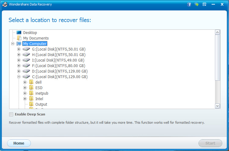
2. Step 2: For the Flash Drive Data Recovery, make sure that the particular USB flash-drive is connected to the computer, and then choose locations where you want to perform the ‘Deep Scan’.

Wondershare Data Recovery Software

3. Step 3: The Scanning operation will then be concluded with a preview of all the lost/deleted files from the USB Flash Drive. Select the files you wish to recover and save them to a fresh location.

Wondershare Data Recovery Software

Conclusion

The Wondershare Data Recovery software is absolutely effective and can perform all the recovery functions without any tech support. One can easily follow the instructions by the software and recover his/her lost files without any difficulties.

The post Wondershare Data Recovery Software appeared first on The Crazy Programmer.

Android Glide Tutorial with Example

$
0
0

Here you will get android glide tutorial with example.

Glide is an android library that allows us to fetch image from internet or url in single line of code. In one of my previous tutorial I have shown you the usage of picasso image library. Glide is a good alternative of Picasso library. Most of the features are common in both of them.

Glide is popular android image library which is recommended by Google and even Google used it in various applications. Below are some features of this library.

Android Glide Tutorial with Example

Features of Glide Image Library

  • Supports fetching of images, gifs and video stills.
  • Placeholder and error image can be added.
  • Support disk caching.
  • Image resize and cropping.

One of the biggest advantage of Glide over Picasso is that Glide supports gifs.

Android Glide Tutorial

Lets quickly jump to the actual tutorial part.

How to fetch image using Glide?

For this you just have to use one line of code given below.

Glide.with(context).load(IMAGE_URL).into(imageView);

Placeholder and Error Image

You can add a placeholder image until the image loaded from internet. You can also add an error image in case any error occurs while fetching image.

Glide.with(context)
	.load(IMAGE_URL)
	.placeholder(R.drawable.PLACEHOLDER_IMAGE_NAME)
	.error(R.drawable.ERROR_IMAGE_NAME)
	.into(imageView);

Loading GIFs

You can load a gif by just adding asGif() method.

Glide.with(context)
	.load(IMAGE_URL)
	.asGif()
	.into(imageView);

Resizing and Cropping Image

The following line of code resizes image to 300×300 pixel and make it center cropped.

Glide.with(context)
	.load(IMAGE_URL)
	.override(200, 200)
	.centerCrop()     
	.into(imageView);

Android Glide Example

Lets make a simple android app that shows the usage of Glide image library.

1. Create an android studio project with package name com.androidglide

2. Now include Glide library to your project by adding following line of code under dependencies section in app level build.gradle file.

compile 'com.github.bumptech.glide:glide:3.7.0'

3. Add internet access permission in AndroidManifest.xml file.

<uses-permission android:name="android.permission.INTERNET"/>

4. Add following code in respective files.

activity_main.xml

<?xml version="1.0" encoding="utf-8"?>
<LinearLayout xmlns:android="http://schemas.android.com/apk/res/android"
    xmlns:app="http://schemas.android.com/apk/res-auto"
    xmlns:tools="http://schemas.android.com/tools"
    android:layout_width="match_parent"
    android:layout_height="match_parent"
    tools:context="com.androidglide.MainActivity"
    android:orientation="vertical">

    <Button
        android:layout_width="match_parent"
        android:layout_height="wrap_content"
        android:text="Load Image"
        android:id="@+id/button"
        android:layout_marginBottom="5dp"/>

    <ImageView
        android:layout_width="match_parent"
        android:layout_height="wrap_content"
        android:id="@+id/image"/>

</LinearLayout>

MainActivity.java

package com.androidglide;

import android.support.v7.app.AppCompatActivity;
import android.os.Bundle;
import android.view.View;
import android.widget.Button;
import android.widget.ImageView;

import com.bumptech.glide.Glide;

public class MainActivity extends AppCompatActivity {
    String IMAGE_URL = "http://www.thecrazyprogrammer.com/wp-content/uploads/2015/09/Neeraj-Mishra.png";
    Button button;
    ImageView image;

    @Override
    protected void onCreate(Bundle savedInstanceState) {
        super.onCreate(savedInstanceState);
        setContentView(R.layout.activity_main);

        button = (Button)findViewById(R.id.button);
        image = (ImageView)findViewById(R.id.image);

        //load image on button click
        button.setOnClickListener(new View.OnClickListener() {
            @Override
            public void onClick(View v) {
                Glide.with(MainActivity.this).load(IMAGE_URL).into(image);
            }
        });
    }
}

5. Save and run the project.

The image is fetched from internet on button click, see below screenshot.

Screenshot

Android Glide Tutorial with Example

Comment below if you have any queries related to above glide android tutorial.

The post Android Glide Tutorial with Example appeared first on The Crazy Programmer.

Sliding Window Protocol Program in C and C++

$
0
0

Here you will get sliding window protocol program in C.

In computer networks sliding window protocol is a method to transmit data on a network. Sliding window protocol is applied on the Data Link Layer of OSI model. At data link layer data is in the form of frames. In Networking, Window simply means a buffer which has data frames that needs to be transmitted.

Both sender and receiver agrees on some window size. If window size=w then after sending w frames sender waits for the acknowledgement (ack) of the first frame.

As soon as sender receives the acknowledgement of a frame it is replaced by the next frames to be transmitted by the sender. If receiver sends a collective or cumulative acknowledgement to sender then it understands that more than one frames are properly received, for eg:- if ack of frame 3 is received it understands that frame 1 and frame 2 are received properly.

Sliding Window Protocol

Image Source

In sliding window protocol the receiver has to have some memory to compensate any loss in transmission or if the frames are received unordered.

Efficiency of Sliding Window Protocol

η = (W*tx)/(tx+2tp)

W = Window Size

tx = Transmission time

tp = Propagation delay

Sliding window works in full duplex mode

It is of two types:-

1. Selective Repeat: Sender transmits only that frame which is erroneous or is lost.

2. Go back n: Sender transmits all frames present in the window that occurs after the error bit including error bit also.

Sliding Window Protocol Program in C

Below is the simulation of sliding window protocol in C.

#include<stdio.h>

int main()
{
    int w,i,f,frames[50];

    printf("Enter window size: ");
    scanf("%d",&w);

    printf("\nEnter number of frames to transmit: ");
    scanf("%d",&f);

    printf("\nEnter %d frames: ",f);

    for(i=1;i<=f;i++)
        scanf("%d",&frames[i]);

    printf("\nWith sliding window protocol the frames will be sent in the following manner (assuming no corruption of frames)\n\n");
    printf("After sending %d frames at each stage sender waits for acknowledgement sent by the receiver\n\n",w);

    for(i=1;i<=f;i++)
    {
        if(i%w==0)
        {
            printf("%d\n",frames[i]);
            printf("Acknowledgement of above frames sent is received by sender\n\n");
        }
        else
            printf("%d ",frames[i]);
    }

    if(f%w!=0)
        printf("\nAcknowledgement of above frames sent is received by sender\n");

    return 0;
}

Output

Enter window size: 3

Enter number of frames to transmit: 5

Enter 5 frames: 12 5 89 4 6

With sliding window protocol the frames will be sent in the following manner (assuming no corruption of frames)

After sending 3 frames at each stage sender waits for acknowledgement sent by the receiver

12 5 89
Acknowledgement of above frames sent is received by sender

4 6
Acknowledgement of above frames sent is received by sender

Sliding Window Protocol Program in C++

Below is the simulation of sliding window protocol in C++.

#include<iostream>

using namespace std;

int main()
{
    int w,i,f,frames[50];

    cout<<"Enter window size: ";
    cin>>w;

    cout<<"\nEnter number of frames to transmit: ";
    cin>>f;

    cout<<"\nEnter "<<f<<" frames: ";

    for(i=1;i<=f;i++)
        cin>>frames[i];

    cout<<"\nWith sliding window protocol the frames will be sent in the following manner (assuming no corruption of frames)\n\n";
    cout<<"After sending "<<w<<" frames at each stage sender waits for acknowledgement sent by the receiver\n\n";

    for(i=1;i<=f;i++)
    {
        if(i%w==0)
        {
            cout<<frames[i]<<"\n";
            cout<<"Acknowledgement of above frames sent is received by sender\n\n";
        }
        else
            cout<<frames[i]<<" ";
    }

    if(f%w!=0)
        cout<<"\nAcknowledgement of above frames sent is received by sender\n";

    return 0;
}

Comment below if you have any queries regarding above program.

The post Sliding Window Protocol Program in C and C++ appeared first on The Crazy Programmer.

Python Program to Check Armstrong Number

$
0
0

Here you will get python program to check armstrong number.

A number is said to be an armstrong number if sum of its digits raised to the power n is equal to itself. Here n is total digits in number.

For example 370 is armstrong number.

Here n = 3, so 33 + 7+ 0= 27 + 343 + 0 = 370

Python Program to Check Armstrong Number

num = int(input("enter a number: "))

length = len(str(num))
sum = 0
temp = num

while(temp != 0):
	sum = sum + ((temp % 10) ** length)
	temp = temp // 10

if sum == num:
	print("armstrong number")
else:
	print("not armstrong number")

Output

enter a number: 370
armstrong number

Comment below if you have any queries related to above program for armstrong number in python.

The post Python Program to Check Armstrong Number appeared first on The Crazy Programmer.

Analysis of Algorithms

$
0
0

In this tutorial you will learn about analysis of algorithms.

Before learning analysis of algorithms lets quickly take a look on what is an algorithm and why we require it.

What is an Algorithm?

An algorithm is the step by step unambiguous procedure to solve a given problem.

For example steps for making Tea or Coffee can be considered as an algorithm.

So for solving a problem we require an algorithm.

Analysis of Algorithms

Design and Analysis of Algorithms

Image Source

There can be several algorithms for solving one problem. So analysis of algorithms is required to find the correctness (algorithm should give solution of problem in finite number of steps) and efficiency (time and memory it takes) of an algorithm.

For example: To go from city A to B there can be several ways like by bus, train, flight, etc.  Depending upon the availability and convenience we choose the one that suits best for us.

Similarly in computer science we use analysis of algorithms to choose the algorithm which is most efficient in terms of running time and space required.

Running Time Analysis

It is the process of determining how processing time of an algorithm increase as the input size increase.

Input size is the number of elements in the input. There can be different types of inputs depending upon the problem type. Below are some common types of inputs.

  • Size of an array.
  • Number of elements in matrix.
  • Vertices and edges in a graph.

Types of Analysis

To analyze an algorithm we need to know for which input the algorithm takes less time and for which input it takes long time.

In terms of running time there can be three cases mentioned below.

Worst Case: It defines the input for which the algorithm takes longest time (slowest time) to complete.

Best Case: It defines the input for which the algorithm takes least time (fastest time) to complete.

Average Case: Run the algorithm using different random inputs and then find total running time by finding average of all running times.

Comment below if have any queries regarding above tutorial.

The post Analysis of Algorithms appeared first on The Crazy Programmer.

Python Program to Convert Decimal to Binary, Octal and Hexadecimal

$
0
0

Here you will get python program to convert decimal to binary, octal and hexadecimal.

Python provides inbuilt functions for conversion of one number system to another.

  • Convert decimal to binary using bin() function. In converted binary form 0b is present at the beginning.
  • Convert decimal to octal using oct() function. In converted octal form 0o is present at the beginning.
  • Convert decimal to hexadecimal using hex() function. In converted hexadecimal form 0x is present at the beginning.

Below program demonstrates that how we can do these conversions.

Python Program to Convert Decimal to Binary, Octal and Hexadecimal

num = int(input("enter a decimal number: "))

print("\nbinary form is ", bin(num))
print("octal form is ", oct(num))
print("hexadecimal form is ", hex(num))

Output

enter a decimal number: 11

binary form is 0b1011
octal form is 0o13
hexadecimal form is 0xb

Comment below if you have any queries regarding above program.

The post Python Program to Convert Decimal to Binary, Octal and Hexadecimal appeared first on The Crazy Programmer.


Python Program to Check Palindrome Number

$
0
0

Here you will get python program to check palindrome number.

A number is said to be palindrome if it is equal to its reverse. For example 121, 555, etc are palindrome while 124, 367, etc are not.

Python Program to Check Palindrome Number

num = int(input("enter a number: "))

temp = num
rev = 0

while temp != 0:
	rev = (rev * 10) + (temp % 10)
	temp = temp // 10

if num == rev:
	print("number is palindrome")
else:
	print("number is not palindrome")

Output

enter a number: 12321
number is palindrome

Comment below if you have any queries regarding python palindrome number program.

The post Python Program to Check Palindrome Number appeared first on The Crazy Programmer.

Difference between Recursion and Iteration

$
0
0

In this tutorial you will learn about difference between recursion and iteration with example.

Both recursion and iteration are used for executing some instructions repeatedly until some condition is true. A same problem can be solved with recursion as well as iteration but still there are several differences in their working and performance that I have mentioned below.

Difference between Recursion and Iteration

  Recursion Iteration
Definition Recursion refers to a situation where a function calls itself again and again until some base condition is not reached. Iteration refers to a situation where some statements are executed again and again using loops until some condition is true.
Performance It is comparatively slower because before each function call the current state of function is stored in stack. After the return statement the previous function state is again restored from stack. Its execution is faster because it doesn’t use stack.
Memory Memory usage is more as stack is used to store the current function state. Memory usage is less as it doesn’t use stack.
Code Size Size of code is comparatively smaller in recursion. Iteration makes the code size bigger.

Lets write the implementation of finding factorial of number using recursion as well as iteration.

Recursion Example

Below is the C program to find factorial of a number using recursion.

#include <stdio.h>

int factorial(int n){
    if(n == 0)
        return 1;
    else
        return n * factorial(n-1);
}

int main() {
    printf("Factorial for 5 is %d", factorial(5));

    return 0;
}

Iteration Example

Below is the C program to find factorial of a number using iteration.

#include <stdio.h>

int main() {
    int i, n = 5, fac = 1;

    for(i = 1; i <= n; ++i)
        fac = fac * i;

    printf("Factorial for 5 is %d", fac);

    return 0;
}

Comment below if you have any queries regarding above tutorial for recursion vs iteration.

The post Difference between Recursion and Iteration appeared first on The Crazy Programmer.

Null Pointer in C

$
0
0

In this tutorial you will learn about null pointer in C with examples.

When we declare a pointer, by default it points to some random memory location. If you will access the pointer then it may give some undesired value or the program may crash.

What is Null Pointer in C?

Null Pointer

A pointer pointing to nothing or no memory location is called null pointer. For doing this we simply assign NULL to the pointer.

So while declaring a pointer we can simply assign NULL to it in following way.

int *p = NULL;

NULL is a constant which is already defined in C and its value is 0. So instead of assigning NULL to pointer while declaring it we can also assign 0 to it.

Usage of Null Pointer

1. We can simply check the pointer is NULL or not before accessing it. This will prevent crashing of program or undesired output.

int *p = NULL;

if(p != NULL) {
//here you can access the pointer
}

2. A pointer pointing to a memory location even after its deallocation is called dangling pointer. When we try to access dangling pointer it crashes the program. So to solve this problem we can simply assign NULL to it.

void function(){
    int *ptr = (int *)malloc(SIZE);
    . . . . . .
    . . . . . . 
    free(ptr);    //ptr now becomes dangling pointer which is pointing to dangling reference
    ptr=NULL;    //now ptr is not dangling pointer
}

3. We can simply pass NULL to a function if we don’t want to pass a valid memory location.

void fun(int *p) {
    //some code
}

int main() {

    fun(NULL);

    return 0;
}

4. Null pointer is also used to represent the end of a linked list.

Linked List

Image Source

Comment below if you found anything incorrect or have queries regarding above tutorial for null pointer in C.

The post Null Pointer in C appeared first on The Crazy Programmer.

Python Linear Search

$
0
0

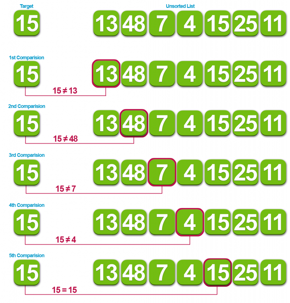
Here you will get program for linear search in python.

Linear search is one of the simplest searching algorithm in which targeted item in sequentially matched with each item in a list. It is worst searching algorithm with worst case time complexity O (n).

Below is its implementation.

Linear Search

Image Source

Program for Python Linear Search

items = [5, 7, 10, 12, 15]

print("list of items is", items)

x = int(input("enter item to search:"))

i = flag = 0

while i < len(items):
	if items[i] == x:
		flag = 1
		break

	i = i + 1

if flag == 1:
	print("item found at position:", i + 1)
else:
	print("item not found")

Output

list of items is [5, 7, 10, 12, 15]
enter item to search:12
item found at position: 4

Comment below if you have any queries regarding python linear search program.

The post Python Linear Search appeared first on The Crazy Programmer.

Travelling Salesman Problem (TSP)

$
0
0

Here you will learn about Travelling Salesman Problem (TSP) with example and also get a program that implements Travelling Salesman Problem in C.

Let say there are some villages (1, 2, 3, 4, 5). To work with worst case let assume each villages connected with every other villages. And there is a Salesman living in village 1 and he has to sell his things in all villages by travelling and he has to come back to own village 1.

He has to travel each village exactly once, because it is waste of time and energy that revisiting same village. This is same as visiting each node exactly once, which is Hamiltonian Circuit. But our problem is bigger than Hamiltonian cycle because this is not only just finding Hamiltonian path, but also we have to find shortest path.

Finally the problem is we have to visit each vertex exactly once with minimum edge cost in a graph.

Brute Force Approach takes O (nn) time, because we have to check (n-1)! paths (i.e all permutations) and have to find minimum among them.

The correct approach for this problem is solving using Dynamic Programming.

Dynamic Programming can be applied only if main problem can be divided into sub-problems. Let’s check that.

Travelling Salesman Problem (TSP) Using Dynamic Programming

Example Problem

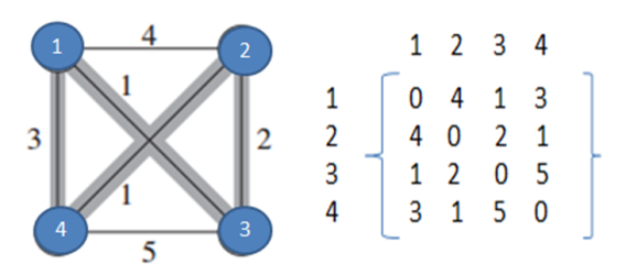
Travelling Salesman Problem (TSP)

Above we can see a complete directed graph and cost matrix which includes distance between each village. We can observe that cost matrix is symmetric that means distance between village 2 to 3 is same as distance between village 3 to 2.

Here problem is travelling salesman wants to find out his tour with minimum cost.

Say it is T (1,{2,3,4}), means, initially he is at village 1 and then he can go to any of {2,3,4}. From there to reach non-visited vertices (villages) becomes a new problem. Here we can observe that main problem spitted into sub-problem, this is property of dynamic programming.

Note: While calculating below right side values calculated in bottom-up manner. Red color values taken from below calculations.

T ( 1, {2,3,4} ) = minimum of

= { (1,2) + T (2,  {3,4} )     4+6=10

= { (1,3)  + T (3, {2,4} )     1+3=4

= { (1,4) + T (4, {2,3} )     3+3=6

Here minimum of above 3 paths is answer but we know only values of (1,2) , (1,3) , (1,4) remaining thing which is T ( 2, {3,4} ) …are new problems now. First we have to solve those and substitute here.

T (2, {3,4} )   = minimum of

=  { (2,3) + T (3, {4} )     2+5=7

= { (2,4) + T {4, {3} )     1+5=6

T (3, {2,4} )   = minimum of

=  { (3,2) + T (2, {4} )     2+1=3

= { (3,4) + T {4, {2} )     5+1=6

T (4, {2,3} )   = minimum of

=  { (4,2) + T (2, {3} )     1+2=3

= { (4,3) + T {3, {2} )     5+2=7

T ( 3, {4} ) =  (3,4) + T (4, {} )     5+0=5

T ( 4, {3} ) =  (4,3) + T (3, {} )     5+0=5

T ( 2, {4} ) =  (2,4) + T (4, {} )     1+0=1

T ( 4, {2} ) =  (4,2) + T (2, {} )     1+0 = 1

T ( 2, {3} ) =  (2,3) + T (3, {} )     2+0 = 2

T ( 3, {2} ) =  (3,2) + T (2, {} )     2+0=2

Here T ( 4, {} ) is reaching base condition in recursion, which returns 0 (zero ) distance.

This is where we can find final answer,

T ( 1, {2,3,4} ) = minimum of

= { (1,2) + T (2,  {3,4} )     4+6=10 in this path we have to add +1 because this path ends with 3. From there we have to reach 1 so 3->1 distance 1 will be added total distance is 10+1=11

= { (1,3)  + T (3, {2,4} )     1+3=4 in this path we have to add +3 because this path ends with 3. From there we have to reach 1 so 4->1 distance 3 will be added total distance is 4+3=7

= { (1,4) + T (4, {2,3} )     3+3=6 in this path we have to add +1 because this path ends with 3. From there we have to reach 1 so 3->1 distance 1 will be added total distance is 6+1=7

Minimum distance is 7 which includes path 1->3->2->4->1.

After solving example problem we can easily write recursive equation.

Recursive Equation

T (i , s) = min ( ( i , j) + T ( j , S – { j }) ) ;  S!= Ø   ; j € S ;

S is set that contains non visited vertices

=  ( i, 1 ) ;  S=Ø, This is base condition for this recursive equation.

Here,

T (i, S) means We are travelling from a vertex “i” and have to visit set of non-visited vertices  “S” and have to go back to vertex 1 (let we started from vertex 1).

( i, j ) means cost of path from node i  to node j

If we observe the first recursive equation from a node we are finding cost to all other nodes (i,j) and from that node to remaining using recursion ( T (j , {S-j}))

But it is not guarantee that every vertex is connected to other vertex then we take that cost as infinity. After that we are taking minimum among all so the path which is not connected get infinity in calculation and won’t be consider.

If S is empty that means we visited all nodes, we take distance from that last visited node to node 1 (first node). Because after visiting all he has to go back to initial node.

Time Complexity

Since we are solving this using Dynamic Programming, we know that Dynamic Programming approach contains sub-problems.

Here after reaching ith node finding remaining minimum distance to that ith node is a sub-problem.

If we solve recursive equation we will get total (n-1) 2(n-2)  sub-problems, which is O (n2n).

Each sub-problem will take  O (n) time (finding path to remaining (n-1) nodes).

Therefore total time complexity is O (n2n) * O (n) = O (n22n)

Space complexity is also number of sub-problems which is O (n2n)

Travelling Salesman Problem in C

#include<stdio.h>

int ary[10][10],completed[10],n,cost=0;

void takeInput()
{
	int i,j;

	printf("Enter the number of villages: ");
	scanf("%d",&n);

	printf("\nEnter the Cost Matrix\n");

	for(i=0;i < n;i++)
	{
		printf("\nEnter Elements of Row: %d\n",i+1);

		for( j=0;j < n;j++)
			scanf("%d",&ary[i][j]);

		completed[i]=0;
	}

	printf("\n\nThe cost list is:");

	for( i=0;i < n;i++)
	{
		printf("\n");

		for(j=0;j < n;j++)
			printf("\t%d",ary[i][j]);
	}
}

void mincost(int city)
{
	int i,ncity;

	completed[city]=1;

	printf("%d--->",city+1);
	ncity=least(city);

	if(ncity==999)
	{
		ncity=0;
		printf("%d",ncity+1);
		cost+=ary[city][ncity];

		return;
	}

	mincost(ncity);
}

int least(int c)
{
	int i,nc=999;
	int min=999,kmin;

	for(i=0;i < n;i++)
	{
		if((ary[c][i]!=0)&&(completed[i]==0))
			if(ary[c][i]+ary[i][c] < min)
			{
				min=ary[i][0]+ary[c][i];
				kmin=ary[c][i];
				nc=i;
			}
	}

	if(min!=999)
		cost+=kmin;

	return nc;
}

int main()
{
	takeInput();

	printf("\n\nThe Path is:\n");
	mincost(0); //passing 0 because starting vertex

	printf("\n\nMinimum cost is %d\n ",cost);

	return 0;
}

Output

Enter the number of villages: 4

Enter the Cost Matrix

Enter Elements of Row: 1
0 4 1 3

Enter Elements of Row: 2
4 0 2 1

Enter Elements of Row: 3
1 2 0 5

Enter Elements of Row: 4
3 1 5 0
The cost list is:
0 4 1 3
4 0 2 1
1 2 0 5
3 1 5 0

The Path is:
1—>3—>2—>4—>1

Minimum cost is 7

Comment below if you found any information incorrect or have doubts regarding Travelling Salesman Problem algorithm.


The post Travelling Salesman Problem (TSP) appeared first on The Crazy Programmer.

Matrix Chain Multiplication in C and C++

$
0
0

Here you will learn about Matrix Chain Multiplication with example and also get a program that implements matrix chain multiplication in C and C++.

Before going to main problem first remember some basis.

We know that, to multiply two matrices it is condition that, number of columns in first matrix should be equal to number of rows in second matrix. Let say there are two matrices A and B with dimensions A (2 x 3) and B (3 x 2).

Let’s see an example.

Matrix Chain Multiplication

Above we can see resultant matrix is (2 x 2) matrix i.e. it contains total 4 elements. To calculate each element we did 3 multiplications (which is equal to number of columns in first matrix and number of rows in second matrix). So totally for 4 elements 4*3 = 12 multiplications are required.

In generalized way matrices A (P x Q) and B(Q x R) will result matrix (P x R) which contains P * R elements. To calculate each element need “Q” number of multiplications. Total multiplications needed are P * Q * R

Let’s  try to multiply more than two matrices.

If 3 matrices A, B ,C we can find the final result in two ways (AB)C or A(BC). We get same result in any way since matrix multiplication satisfies associativity property.

Let A (1 x 2 ), B (2 x 3 ), C ( 3 x 2 ). If we follow first way, i.e. (AB)C way.

To calculate (AB) we need 1*2*3 = 6 multiplications. Now resultant AB get dimensions 1 x 3 this multiplied with C need 1*3*2 = 6 multiplications. Total 6+6 = 12 multiplications needed.

If we follow second way, i.e. A(BC) way.

To calculate (BC) we need 2*3*2 = 12 multiplications. Now resultant BC get dimensions 2 x 3. A multiplied with this result need 1*2*3 = 6. Total 12+6 = 18 multiplications needed.

Here we can observe that based on the way we parenthesize the matrices total number of multiplications are changing.

If 4 matrices A, B, C, D we can find final result in 5 ways A(B(CD)) or A((BC)(D)) or (AB)(CD) 4. ((AB)C)D  or (A(BC))D. In this case also each way requires different number of multiplications.

General formula to find number of ways we can find solution is  (2n)! / [ (n+1)! n! ]. After parenthesizing these many ways each way requires different number of multiplications for final result. When dimensions are large (200 x 250 like this) with more number of matrices, then finding the parenthesizing way which requires minimum number of multiplications need will gives less time complexity.

So Matrix Chain Multiplication problem aim is not to find the final result of multiplication, it is finding how to parenthesize matrices so that, requires minimum number of multiplications.

Efficient way of solving this is using dynamic programming

Matrix Chain Multiplication Using Dynamic Programming

Let we have “n” number of matrices A1, A2, A3 ……… An and dimensions are d0 x d1, d1 x d2, d2 x d3 …………. dn-1 x dn  (i.e Dimension of Matrix Ai is di-1 x di

Solving a chain of matrix that,  Ai  Ai+1  Ai+2  Ai+3 ……. Aj = (Ai  Ai+1  Ai+2  Ai+3 ……. Ak ) (Ak+1  Ak+2 ……. Aj ) + di-1 dk dj where i <= k < j.

For more understanding check below example.

Here total i to j matrices, Matrix i to k and Matrix k+1 to j should be solved in recursive way and finally these two matrices multiplied and these dimensions di-1 dk dj (number of multiplications needed) added. The variable k is changed i to j.

Recursive Equation

Note: M[i, j] indicates that if we split from matrix i to matrix j then minimum number of scalar multiplications required.

M [ i , j ] = { 0 ; when i=j ; [means it is a single matrix . If there is only one matrix no need to multiply  with any other. So 0 (zero) multiplications required.]

= { min { M[ i, k ] + M[k+1, j  ] + di-1 dk dj } where i <= k< j

Example Problem

Given problem: A1 (10 x 100), A2 (100 x 20), A3(20 x 5), A4 (5 x 80)

To store results, in dynamic programming we create a table

1,1=0 2,2=0 3,3=0 4,4=0
1,2=20000 2,3=10000 3,4=8000
1,3=15000 2,4=50000
1,4=19000

This table filled using below calculations.

Here cell 2,3 stores the minimum number of scalar multiplications required to.

Using above recursive equation we can fill entire first row with all 0’s (zeros) because i=j (i.e. split happened at only one matrix which requires zero multiplications)

Table [1,2] = 10*100*20 = 20000

Table [2,3] = 100*20*5 = 10000

Table [3,4] = 20*5*80 = 8000

Table [1,3] = minimum of

= { (1,1) + (2,3) + 10* 100*5  = 0+10000+5000 = 15000

= { (1,2) + (3,3) + 10*20*5 = 20000+0+1000 = 21000

Therefore Table[1,3] is 15000 and split happened at 1

Table [2,4] = minimum of

= { (2,2) +(3,4) + 100*20*80 = 0 + 8000 + 160000 = 168000

= { (2,3) + (4,4) + 100*5*80 = 10000 + 0 + 40000 = 50000

Therefore Table of [2,4] is 50000 and split happened at 3

Table of [1,4] = minimum of

= { (1,1) +(2,4) + 10*100*80 = 0 + 50000 + 80000 = 130000

= { (1,2) +(3,4) + 10* 20* 80 = 20000 + 8000 + 16000 = 44000

= { (1,3) + (4,4) + 10*5*80 = 15000+0+4000 = 19000

Therefore table of [1,4] is 19000 which is final answer and split happened at 3.

Splitting way: (1234) is original in final outcome where 19000 answer we got split happened at 3 so ( 1 2 3 ) (4). Split for (123) means see at Table [1,3] that one minimum 15000 split at 1 . So ( ( 1 ) ( 2 3 ) ) ( 4). That means first do 2 x 3 and this 1 x first result and then this result x 4.

Time Complexity

If there are n number of matrices we are creating a table contains [(n) (n+1) ] / 2 cells that is in worst case total number of cells n*n = n2 cells we need calculate = O (n2)

For each one of entry we need find minimum number of multiplications taking worst (it happens at  last cell in table) that is Table [1,4] which equals to  O (n) time.

Finally O (n2) * O (n) = O (n3) is time complexity.

Space Complexity

We are creating a table of n x n so space complexity is O (n2).

Program for Matrix Chain Multiplication in C

// This code implemented using Algorithm in Coremen book

#include<stdio.h>
#include<limits.h>

// Matrix Ai has dimension p[i-1] x p[i] for i = 1..n

int MatrixChainMultiplication(int p[], int n)
{
    int m[n][n];
    int i, j, k, L, q;

    for (i=1; i<n; i++)
        m[i][i] = 0;    //number of multiplications are 0(zero) when there is only one matrix

    //Here L is chain length. It varies from length 2 to length n.
    for (L=2; L<n; L++)
    {
        for (i=1; i<n-L+1; i++)
        {
            j = i+L-1;
            m[i][j] = INT_MAX;  //assigning to maximum value

            for (k=i; k<=j-1; k++)
            {
                q = m[i][k] + m[k+1][j] + p[i-1]*p[k]*p[j];
                if (q < m[i][j])
                {
                    m[i][j] = q;    //if number of multiplications found less that number will be updated.
                }
            }
        }
    }

    return m[1][n-1];   //returning the final answer which is M[1][n]

}

int main()
{
    int n,i;
    printf("Enter number of matrices\n");
    scanf("%d",&n);

    n++;

    int arr[n];

    printf("Enter dimensions \n");

    for(i=0;i<n;i++)
    {
        printf("Enter d%d :: ",i);
        scanf("%d",&arr[i]);
    }

    int size = sizeof(arr)/sizeof(arr[0]);

    printf("Minimum number of multiplications is %d ", MatrixChainMultiplication(arr, size));

    return 0;
}

Output

Enter number of matrices
4
Enter dimensions
Enter d0 :: 10
Enter d1 :: 100
Enter d2 :: 20
Enter d3 :: 5
Enter d4 :: 80
Minimum number of multiplications is 19000

Program for Matrix Chain Multiplication in C++

// This code implemented using Algorithm in Coremen book

#include<iostream>
#include<limits.h>

using namespace std;

// Matrix Ai has dimension p[i-1] x p[i] for i = 1..n

int MatrixChainMultiplication(int p[], int n)
{
    int m[n][n];
    int i, j, k, L, q;

    for (i=1; i<n; i++)
        m[i][i] = 0;    //number of multiplications are 0(zero) when there is only one matrix

    //Here L is chain length. It varies from length 2 to length n.
    for (L=2; L<n; L++)
    {
        for (i=1; i<n-L+1; i++)
        {
            j = i+L-1;
            m[i][j] = INT_MAX;  //assigning to maximum value

            for (k=i; k<=j-1; k++)
            {
                q = m[i][k] + m[k+1][j] + p[i-1]*p[k]*p[j];
                if (q < m[i][j])
                {
                    m[i][j] = q;    //if number of multiplications found less that number will be updated.
                }
            }
        }
    }

    return m[1][n-1];   //returning the final answer which is M[1][n]

}

int main()
{
    int n,i;
    cout<<"Enter number of matrices\n";
    cin>>n;

    n++;

    int arr[n];

    cout<<"Enter dimensions \n";

    for(i=0;i<n;i++)
    {
        cout<<"Enter d"<<i<<" :: ";
        cin>>arr[i];
    }

    int size = sizeof(arr)/sizeof(arr[0]);

    cout<<"Minimum number of multiplications is "<<MatrixChainMultiplication(arr, size));

    return 0;
}

Comment below if you have any queries related to above program for matrix chain multiplication in C and C++.

The post Matrix Chain Multiplication in C and C++ appeared first on The Crazy Programmer.

Topological Sort in C and C++

$
0
0

Here you will learn and get program for topological sort in C and C++.

We know many sorting algorithms used to sort the given data. It may be numeric data or strings. Take a situation that our data items have relation. They are related with some condition that one should happen only after other one happened.

For example shoe should wear after socks only. Another example, in academic course one should study Applications of Algorithms subject only after studying Designing of Algorithms. And Designing of Algorithms should study only after learning any programming language. We can observe that a work requires pre-requisite. In these situations we represent our data in a graph and we use directed edges from pre-requisite to next one. And we apply Topological sorting to solve.

Most important condition to do Topological sorting on any graph is that Graph should be Connected Directed Acyclic graph. It is not possible to apply Topological sorting either graph is not directed or it have a Cycle.

One more condition is that graph should contain a sink vertex. The vertex which doesn’t have any outgoing edge is called sink vertex. Idea behind this sink vertex is that if every vertex has an outgoing edge in a directed graph it definitely forms a cycle, which violates the condition.

Note: Topological sorting on a graph results non-unique solution

Topological Sort Example

Topological Sort in C and C++

Solving Using In-degree Method

Step 1: Write in-degree of all vertices:

Vertex in-degree
1 0
2 1
3 1
4 2

Step 2: Write the vertex which has in-degree 0 (zero) in solution. Here vertex 1 has in-degree 0. So,

Solution is: 1 -> (not yet completed )

Decrease in-degree count of vertices who are adjacent to the vertex which recently added to the solution.

Here vertex 1 is recently added to the solution. Vertices 2 and 3 are adjacent to vertex 1. So decrease the in-degree count of those and update.

Updated result is:

Vertex in-degree
1 Already added to solution
2 0
3 0
4 2

Again repeat the same thing which we have done in step1 that, write the vertices which have degree 0 in solution.

Here we can observe that two vertices (2 and 3) have in-degree 0 (zero). Add any vertex into the solution.

Note that, you may add vertex 2 into solution, and I may add vertex 3 to solution. That means the solution to topological sorting is not unique.

Now add vertex 3.

Solution is: 1->3->

Again decrease the in-degree count of vertices which are adjacent to vertex 3.

Updated result is:

Vertex in-degree
1 Already added to solution
2 0
3 Already added to solution
4 1

Now add vertex 2 to solution because it only has in-degree 0.

Solution is: 1->3->2->

Updated result is:

Vertex in-degree
1 Already added to solution
2 Already added to solution
3 Already added to solution
4 0

Finally add 4 to solution.

Final solution is: 1->3->2->4

Program for Topological Sort in C

#include <stdio.h>

int main(){
	int i,j,k,n,a[10][10],indeg[10],flag[10],count=0;

	printf("Enter the no of vertices:\n");
	scanf("%d",&n);

	printf("Enter the adjacency matrix:\n");
	for(i=0;i<n;i++){
		printf("Enter row %d\n",i+1);
		for(j=0;j<n;j++)
			scanf("%d",&a[i][j]);
	}

	for(i=0;i<n;i++){
        indeg[i]=0;
        flag[i]=0;
    }

    for(i=0;i<n;i++)
        for(j=0;j<n;j++)
            indeg[i]=indeg[i]+a[j][i];

    printf("\nThe topological order is:");

    while(count<n){
        for(k=0;k<n;k++){
            if((indeg[k]==0) && (flag[k]==0)){
                printf("%d ",(k+1));
                flag [k]=1;
            }

            for(i=0;i<n;i++){
                if(a[i][k]==1)
                    indeg[k]--;
            }
        }

        count++;
    }

    return 0;
}

Output

Enter the no of vertices:
4
Enter the adjacency matrix:
Enter row 1
0 1 1 0
Enter row 2
0 0 0 1
Enter row 3
0 0 0 1
Enter row 4
0 0 0 0

The topological order is:1 2 3 4

Program for Topological Sort in C++

#include<iostream>

using namespace std;

int main(){
	int i,j,k,n,a[10][10],indeg[10],flag[10],count=0;

	cout<<"Enter the no of vertices:\n";
	cin>>n;

	cout<<"Enter the adjacency matrix:\n";
	for(i=0;i<n;i++){
		cout<<"Enter row "<<i+1<<"\n";
		for(j=0;j<n;j++)
			cin>>a[i][j];
	}

	for(i=0;i<n;i++){
        indeg[i]=0;
        flag[i]=0;
    }

    for(i=0;i<n;i++)
        for(j=0;j<n;j++)
            indeg[i]=indeg[i]+a[j][i];

    cout<<"\nThe topological order is:";

    while(count<n){
        for(k=0;k<n;k++){
            if((indeg[k]==0) && (flag[k]==0)){
                cout<<k+1<<" ";
                flag[k]=1;
            }

            for(i=0;i<n;i++){
                if(a[i][k]==1)
                    indeg[k]--;
            }
        }

        count++;
    }

    return 0;
}

Comment below if you have any queries related to above program for topological sort in C and C++.


The post Topological Sort in C and C++ appeared first on The Crazy Programmer.


Bellman-Ford Algorithm in C and C++

$
0
0

Here you will learn about Bellman-Ford Algorithm in C and C++.

Dijkstra and Bellman-Ford Algorithms used to find out single source shortest paths. i.e. there is a source node, from that node we have to find shortest distance to every other node. Dijkstra algorithm fails when graph has negative weight cycle. But Bellman-Ford Algorithm won’t fail even, the graph has negative edge cycle. If there any negative edge cycle it will detect and say there is negative edge cycle. If not it will give answer to given problem.

Bellman-Ford Algorithm will work on logic that, if graph has n nodes, then shortest path never contain more than n-1 edges. This is exactly what Bellman-Ford do. It is enough to relax each edge (v-1) times to find shortest path. But to find whether there is negative cycle or not we again do one more relaxation. If we get less distance in nth relaxation we can say that there is negative edge cycle. Reason for this is negative value added and distance get reduced.

Relaxing edge

In algorithm and code below we use this term Relaxing edge.

Relaxing edge is an operation performed on an edge (u, v) . when,

d(u) > d(v) + Cost(u,v)

Here d(u) means distance of u. If already known distance to “u” is greater than the path from “s” to “v” and “v” to “u” we update that d(u) value with d(v) + cost(u,v).

Algorithm and Time Complexity

Bellman-Ford (G,w,S){   //G is graph given, W is weight matrix, S is source vertex (starting vertex)
    Initialize single source (G,S)  //means initially distance to every node is infinity except to source. Source is 0 (zero). This will take O(v) time

    For i=1 to |G.V| -1     //Runs (v-1) times
        For each edge (G,V)€ G.E    // E times
            Relax(u,v,w)    //O(1) time

    For each edge (G,V) € G.E
        If (v.d > u.d + w(u,v))     //The idea behind this is we are relaxing edges nth time if we found more shortest path than (n-1)th level, we can say that graph is having negative edge cycle and detected.
            Return False

    return true
}

Finally time complexity is (v-1) (E) O(1) = O(VE)

Example Problem

Bellman-Ford Algorithm 1

This is the given directed graph.

(s,t) = 6  (y,x) = -3

(s,y)= 7  (y,z) = 9

(t,y) = 8  (x,t) = -2

(t,z) = -4  (z,x) = 7

(t,x) = 5  (z,s) = 2

Above we can see using vertex “S” as source (Setting distance as 0), we initialize all other distance as infinity.

  S T X Y Z
distance 0
Path

Table and Image explanation: This table, 2nd row shows distance from source to that particular node ad 3rd row shows to reach that node what is the node we visited recently. This path we can see in the image also.

Note: In each iteration, iteration “n” means it contains the path at most “n” edges. And while we are doing iteration “n” we must follow the graph which we obtained in iteration “n-1”.

Iteration 1: edge (s,t) and (z,y) relaxed and updating the distances to t and y.

Bellman-Ford Algorithm

  S T X Y Z
distance 0 6 7
Path S S

Iteration 2 : edge (t,z) and (y,x) relaxed and x and z values are updated.

Bellman-Ford Algorithm 3

  S T X Y Z
distance 0 6 4 7 2
Path S Y S T

Iteration 3: Value of t updated by relaxing (x,t)

Bellman-Ford Algorithm 4

  S T X Y Z
distance 0 2 4 7 2
Path X Y S T

Iteration 4: Value of z updated by relaxing edge (t,z)

Bellman-Ford Algorithm 5

Until now 4 iterations completed and shortest path found to every node form source node. Now we have to do one more iteration to find whether there exists negative edge cycle or not. When we do this nth (5th here) relaxation if we found less distance to any vertex from any other path we can say that there is negative edge cycle. Here we can relax any edge to graph which obtained in iteration 4and we can observe that there is no chance to change those values. So we can confirm that there is no negative edge cycle in this graph.

Program for Bellman-Ford Algorithm in C

Code explanation

Bellman-Ford Algorithm 6

This picture shows the Structure of our input graph.

We create a structure called “Graph” which contains two integers int v (represent number of vertices) and int E (represents number of edges) and also another structure inside this structure which represents edge. That structure contains 3 integers source, destination, weight of that edge. So we create “E” number of structures inside the structure Graph.

After creating Graph, choose a source node and send to BellmanFord function. In this function we relax each edge “v-1” times. After this we can store the result of shortest paths in an array. And we do one more relaxation to find whether there exists negative edge cycle or not. If we got less distance at any node in Vth relaxation of edges, then we can say that the graph have negative edge cycle.

#include <stdio.h>
#include <stdlib.h>
#include <string.h>
#include <limits.h>

struct Edge
{
    // This structure is equal to an edge. Edge contains two end points. These edges are directed edges so they
	//contain source and destination and some weight. These 3 are elements in this structure
    int source, destination, weight;
};

// a structure to represent a connected, directed and weighted graph
struct Graph
{
    int V, E;
	// V is number of vertices and E is number of edges

    struct Edge* edge;
	// This structure contain another structure which we already created edge.
};

struct Graph* createGraph(int V, int E)
{
    struct Graph* graph = (struct Graph*) malloc( sizeof(struct Graph));
	//Allocating space to structure graph

    graph->V = V;   //assigning values to structure elements that taken form user.

    graph->E = E;

    graph->edge = (struct Edge*) malloc( graph->E * sizeof( struct Edge ) );
	//Creating "Edge" type structures inside "Graph" structure, the number of edge type structures are equal to number of edges

    return graph;
}

void FinalSolution(int dist[], int n)
{
	// This function prints the final solution
    printf("\nVertex\tDistance from Source Vertex\n");
    int i;

    for (i = 0; i < n; ++i){
		printf("%d \t\t %d\n", i, dist[i]);
	}
}

void BellmanFord(struct Graph* graph, int source)
{
    int V = graph->V;

    int E = graph->E;

    int StoreDistance[V];

    int i,j;

    // This is initial step that we know , we initialize all distance to infinity except source.
	// We assign source distance as 0(zero)

    for (i = 0; i < V; i++)
        StoreDistance[i] = INT_MAX;

    StoreDistance[source] = 0;

    //The shortest path of graph that contain V vertices, never contain "V-1" edges. So we do here "V-1" relaxations
    for (i = 1; i <= V-1; i++)
    {
        for (j = 0; j < E; j++)
        {
            int u = graph->edge[j].source;

            int v = graph->edge[j].destination;

            int weight = graph->edge[j].weight;

            if (StoreDistance[u] + weight < StoreDistance[v])
                StoreDistance[v] = StoreDistance[u] + weight;
        }
    }

    // Actually upto now shortest path found. But BellmanFord checks for negative edge cycle. In this step we check for that
    // shortest distances if graph doesn't contain negative weight cycle.

    // If we get a shorter path, then there is a negative edge cycle.
    for (i = 0; i < E; i++)
    {
        int u = graph->edge[i].source;

        int v = graph->edge[i].destination;

        int weight = graph->edge[i].weight;

        if (StoreDistance[u] + weight < StoreDistance[v])
            printf("This graph contains negative edge cycle\n");
    }

    FinalSolution(StoreDistance, V);

    return;
}

int main()
{
    int V,E,S;  //V = no.of Vertices, E = no.of Edges, S is source vertex

	printf("Enter number of vertices in graph\n");
    scanf("%d",&V);

	printf("Enter number of edges in graph\n");
    scanf("%d",&E);

	printf("Enter your source vertex number\n");
	scanf("%d",&S);

    struct Graph* graph = createGraph(V, E);    //calling the function to allocate space to these many vertices and edges

    int i;
    for(i=0;i<E;i++){
        printf("\nEnter edge %d properties Source, destination, weight respectively\n",i+1);
        scanf("%d",&graph->edge[i].source);
        scanf("%d",&graph->edge[i].destination);
        scanf("%d",&graph->edge[i].weight);
    }

    BellmanFord(graph, S);
	//passing created graph and source vertex to BellmanFord Algorithm function

    return 0;
}

Output

Enter number of vertices in graph
5
Enter number of edges in graph
10
Enter your source vertex number
0

Enter edge 1 properties Source, destination, weight respectively
0 1 6

Enter edge 2 properties Source, destination, weight respectively
0 2 7

Enter edge 3 properties Source, destination, weight respectively
1 2 8

Enter edge 4 properties Source, destination, weight respectively
1 4 -4

Enter edge 5 properties Source, destination, weight respectively
1 3 5

Enter edge 6 properties Source, destination, weight respectively
3 1 -2

Enter edge 7 properties Source, destination, weight respectively
2 3 -3

Enter edge 8 properties Source, destination, weight respectively
2 4 9

Enter edge 9 properties Source, destination, weight respectively
4 0 2

Enter edge 10 properties Source, destination, weight respectively
4 3 7

Vertex  Distance from Source Vertex
0  0
1  2
2  7
3  4
4  -2

Program for Bellman-Ford Algorithm in C++

#include <iostream>
#include <stdlib.h>
#include <string.h>
#include <limits.h>

using namespace std;

struct Edge
{
    // This structure is equal to an edge. Edge contains two end points. These edges are directed edges so they
	//contain source and destination and some weight. These 3 are elements in this structure
    int source, destination, weight;
};

// a structure to represent a connected, directed and weighted graph
struct Graph
{
    int V, E;
	// V is number of vertices and E is number of edges

    struct Edge* edge;
	// This structure contain another structure which we already created edge.
};

struct Graph* createGraph(int V, int E)
{
    struct Graph* graph = (struct Graph*) malloc( sizeof(struct Graph));
	//Allocating space to structure graph

    graph->V = V;   //assigning values to structure elements that taken form user.

    graph->E = E;

    graph->edge = (struct Edge*) malloc( graph->E * sizeof( struct Edge ) );
	//Creating "Edge" type structures inside "Graph" structure, the number of edge type structures are equal to number of edges

    return graph;
}

void FinalSolution(int dist[], int n)
{
	// This function prints the final solution
    cout<<"\nVertex\tDistance from Source Vertex\n";
    int i;

    for (i = 0; i < n; ++i){
		cout<<i<<"\t\t"<<dist[i]<<"\n";
	}
}

void BellmanFord(struct Graph* graph, int source)
{
    int V = graph->V;

    int E = graph->E;

    int StoreDistance[V];

    int i,j;

    // This is initial step that we know , we initialize all distance to infinity except source.
	// We assign source distance as 0(zero)

    for (i = 0; i < V; i++)
        StoreDistance[i] = INT_MAX;

    StoreDistance[source] = 0;

    //The shortest path of graph that contain V vertices, never contain "V-1" edges. So we do here "V-1" relaxations
    for (i = 1; i <= V-1; i++)
    {
        for (j = 0; j < E; j++)
        {
            int u = graph->edge[j].source;

            int v = graph->edge[j].destination;

            int weight = graph->edge[j].weight;

            if (StoreDistance[u] + weight < StoreDistance[v])
                StoreDistance[v] = StoreDistance[u] + weight;
        }
    }

    // Actually upto now shortest path found. But BellmanFord checks for negative edge cycle. In this step we check for that
    // shortest distances if graph doesn't contain negative weight cycle.

    // If we get a shorter path, then there is a negative edge cycle.
    for (i = 0; i < E; i++)
    {
        int u = graph->edge[i].source;

        int v = graph->edge[i].destination;

        int weight = graph->edge[i].weight;

        if (StoreDistance[u] + weight < StoreDistance[v])
            cout<<"\nThis graph contains negative edge cycle\n";
    }

    FinalSolution(StoreDistance, V);

    return;
}

int main()
{
    int V,E,S;  //V = no.of Vertices, E = no.of Edges, S is source vertex

	cout<<"Enter number of vertices in graph\n";
    cin>>V;

	cout<<"Enter number of edges in graph\n";
    cin>>E;

	cout<<"Enter your source vertex number\n";
	cin>>S;

    struct Graph* graph = createGraph(V, E);    //calling the function to allocate space to these many vertices and edges

    int i;
    for(i=0;i<E;i++){
        cout<<"\nEnter edge "<<i+1<<" properties Source, destination, weight respectively\n";
        cin>>graph->edge[i].source;
        cin>>graph->edge[i].destination;
        cin>>graph->edge[i].weight;
    }

    BellmanFord(graph, S);
	//passing created graph and source vertex to BellmanFord Algorithm function

    return 0;
}

Reference: Introduction to Algorithms by Thomas H. Cormen

Comment below if you have queries or found anything incorrect in above tutorial for Bellman-Ford Algorithm in C and C++.

The post Bellman-Ford Algorithm in C and C++ appeared first on The Crazy Programmer.
Difference between BFS and DFS

$
0
0

Here you will learn about difference between BFS and DFS algorithm or BFS vs. DFS.

Breadth First Search (BFS) and Depth First Search (DFS) are two popular algorithms to search an element in Graph or to find whether a node can be reachable from root node in Graph or not. And these are popular traversing methods also.

When we apply these algorithms on a Graph, we can see following types of nodes.

  1. Non-Visited nodes: These nodes not yet visited.
  2. Visited nodes: These nodes are visited.
  3. Explored nodes: A node is said to be explored when it was visited and all nodes which are connected (adjacent) to that node also visited.

Difference between BFS and DFS

S. No. Breadth First Search (BFS) Depth First Search (DFS)
1. BFS visit nodes level by level in Graph. DFS visit nodes of graph depth wise. It visits nodes until reach a leaf or a node which doesn’t have non-visited nodes.
2. A node is fully explored before any other can begin. Exploration of a node is suspended as soon as another unexplored is found.
3. Uses Queue data structure to store Un-explored nodes. Uses Stack data structure to store Un-explored nodes.
4. BFS is slower and require more memory. DFS is faster and require less memory.
5. Some Applications:
  • Finding all connected components in a graph.
  • Finding the shortest path between two nodes.
  • Finding all nodes within one connected component.
  • Testing a graph for bipartiteness.
Some Applications:
  • Topological Sorting.
  • Finding connected components.
  • Solving puzzles such as maze.
  • Finding strongly connected components.
  • Finding articulation points (cut vertices) of the graph.

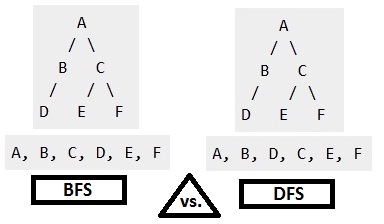
Example

Considering A as starting vertex.

Difference between BFS and DFS

Image Source

Note: There are many sequences possible for BFS and DFS. Using permutations we can find how many are there.

Comment below if you found any information incorrect or missing in above tutorial for difference between dfs and bfs.

The post Difference between BFS and DFS appeared first on The Crazy Programmer.

Hashing in C and C++

$
0
0

In this tutorial you will learn about Hashing in C and C++ with program example. You will also learn various concepts of hashing like hash table, hash function, etc.

Hashing in Data Structure

Searching is dominant operation on any data structure. Most of the cases for inserting, deleting, updating all operations required searching first. So searching operation of particular data structure determines it’s time complexity. If we take any data structure the best time complexity for searching is O (log n) in AVL tree and sorted array only. Most of the cases it will take O (n) time. To solve this searching problem hashing concept introduced which will take O (1) time for searching. It’s constant time.

Hash Table and Hash Function

Earlier when this concept introduced programmers used to create “Direct address table”. Direct address table means, when we have “n” number of unique keys we create an array of length “n” and insert element “i” at ith index of the array. That array is called Hash Table. But due to this method even we have 10 elements of each range 1 lack, we should create table of size 1 lack for only 10 elements. Which is going to be waste of memory.

To avoid this problem we fix the size of hash table (array) and map our elements into that table using a function, called Hash function. This function decides where to put a given element into that table. If we want to search also first apply hash function decide whether the element present in hash table or not.

Example

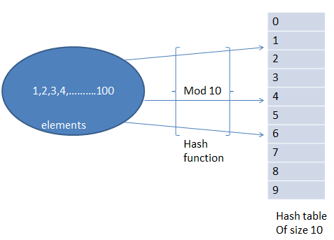
We have numbers from 1 to 100 and hash table of size 10. Hash function is mod 10. That means number 23 will be mapped to (23 mod 10 = 3) 3rd index of hash table.

Hashing, Hash Table, Hash Function

But problem is if elements (for example) 2, 12, 22, 32, elements need to be inserted then they try to insert at index 2 only. This problem is called Collision. To solve this collision problem we use different types of hash function techniques. Those are given below.

  1. Chaining
  2. Open addressing
    1. Linear probing
    2. Quadratic probing
    3. Double hashing

These also called collision resolution techniques.

Chaining

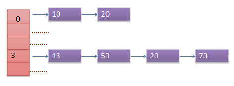
In hash table instead of putting one element in index we maintain a linked list. When collision happened we place that element in corresponding linked list. Here some space is wasted because of pointers.

Hashing 1

Open Addressing

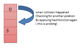
In case if we have collision we again calculate the hash value using corresponding hash function. But this time we do some minor modifications to that input. This process of searching for empty space to insert element in called Probing.

Hashing 2

Probing hash function is: h (k, i)

here k is the key value which is to be inserted. And i is number of collision with that element.

Example: If we are inserting 2, we find its hash value using h (2, 0) because it’s first collision. Suppose the answer (index) to this function index already occupied we again need to apply h (2, 1) to hash function.

Linear Probing

Let hash function is h, hash table contains  0 to n-1 slots.

Now we want to insert an element k. Apply h (k). If it results “x” and the index “x” already contain a value then we again apply hash function that h (k, 1) this equals to (h (k) + 1) mod n.

General form: h1 (k, j) = (h (k) + j) mod n

Example: Let hash table of size 5 which has function is mod 5 has already filled at positions 0, 2, 3.

Now new element 10 will try to insert. 10 mod 5 = 0. But index 0 already occupied. So it checks (probes) next (index 1) position. So 10 will insert at index 1.

Now element 11 will try to insert. 11 mod 5 = 1. But index 1 already occupied, check index 2 it also occupied (data given), 3 also occupied. So it will insert at index 4 which is empty.

We can observe that it linearly checking for next empty position. So it’s called linear probing.

Problems with linear probing:

  • Primary clustering: There is a chance that continuous cells occupied, then the probability of new element insertion will get reduced. This problem is called primary clustering
  • Secondary clustering: If two elements get same value at first hash function, they follow same probe sequence.

Quadratic Probing

It is same as linear probing. But when collision occurs we use different function. If collision happened that element try to occupy at quadratic distance instead of linear distance.

Due to this “Primary clustering” will be reduced. But secondary clustering won’t be eliminated.

Double Hashing

Here we use two hash functions.

h1 (k) = (h1 (k) + i h2 (k)) mod n. Here h1 and h2 are two hash functions.

Here the next prob position will depend on two functions h1 and h2 also.

Advantages by this method are there is no chance of primary clustering. And also Secondary clustering also eliminated.

Chaining vs Open Addressing

Chaining Open Addressing
Elements can be stored at outside of the table In open addressing elements should be stored inside the table only
In chaining at any time the number of elements in the hash table may greater than the size of the hash table In open addressing the number of elements present in the hash table will not exceed to number of indices in hash table.
In case of deletion chaining is the best method If deletion is not required. Only inserting and searching is required open addressing is better
Chaining requires more space Open addressing requires less space than chaining.

Program for Hashing in C

Below is the implementation of hashing or hash table in C.

#include<stdio.h>
#include<limits.h>

/*
This is code for linear probing in open addressing. If you want to do quadratic probing and double hashing which are also
open addressing methods in this code when I used hash function that (pos+1)%hFn in that place just replace with another function.
*/

void insert(int ary[],int hFn, int size){
    int element,pos,n=0;

	printf("Enter key element to insert\n");
	scanf("%d",&element);

	pos = element%hFn;

	while(ary[pos]!= INT_MIN) {  // INT_MIN and INT_MAX indicates that cell is empty. So if cell is empty loop will break and goto bottom of the loop to insert element
		if(ary[pos]== INT_MAX)
            break;
		pos = (pos+1)%hFn;
		n++;
		if(n==size)
		break;      // If table is full we should break, if not check this, loop will go to infinite loop.
	}

	if(n==size)
        printf("Hash table was full of elements\nNo Place to insert this element\n\n");
	else
        ary[pos] = element;    //Inserting element
}

void delete(int ary[],int hFn,int size){
	/*
	very careful observation required while deleting. To understand code of this delete function see the note at end of the program
	*/
	int element,n=0,pos;

	printf("Enter element to delete\n");
	scanf("%d",&element);

	pos = element%hFn;

	while(n++ != size){
		if(ary[pos]==INT_MIN){
			printf("Element not found in hash table\n");
			break;
		}
		else if(ary[pos]==element){
			ary[pos]=INT_MAX;
			printf("Element deleted\n\n");
			break;
		}
		else{
			pos = (pos+1) % hFn;
		}
	}
	if(--n==size)
        printf("Element not found in hash table\n");
}

void search(int ary[],int hFn,int size){
	int element,pos,n=0;

	printf("Enter element you want to search\n");
	scanf("%d",&element);

	pos = element%hFn;

	while(n++ != size){
		if(ary[pos]==element){
			printf("Element found at index %d\n",pos);
			break;
		}
		else
            if(ary[pos]==INT_MAX ||ary[pos]!=INT_MIN)
                pos = (pos+1) %hFn;
	}
	if(--n==size) printf("Element not found in hash table\n");
}

void display(int ary[],int size){
	int i;

	printf("Index\tValue\n");

	for(i=0;i<size;i++)
        printf("%d\t%d\n",i,ary[i]);
}
int main(){
	int size,hFn,i,choice;

	printf("Enter size of hash table\n");
	scanf("%d",&size);

	int ary[size];

	printf("Enter hash function [if mod 10 enter 10]\n");
	scanf("%d",&hFn);

	for(i=0;i<size;i++)
        ary[i]=INT_MIN; //Assigning INT_MIN indicates that cell is empty

	do{
		printf("Enter your choice\n");
		printf(" 1-> Insert\n 2-> Delete\n 3-> Display\n 4-> Searching\n 0-> Exit\n");
		scanf("%d",&choice);

		switch(choice){
			case 1:
				insert(ary,hFn,size);
				break;
			case 2:
				delete(ary,hFn,size);
				break;
			case 3:
				display(ary,size);
				break;
			case 4:
				search(ary,hFn,size);
				break;
			default:
				printf("Enter correct choice\n");
				break;
		}
	}while(choice);

	return 0;
}

/*
Note: Explanation for delete function and search function
suppose hash table contains elements 22, 32, 42 at index positions 2, 3, 4.
Now delete(22) applied. As per hash function defined we first check for index 2. Found, so deleted. And make that index to nill.
Next apply delete(32). This time also it first check at index 2, but found that its nothing.Then we stop and say element 32 not
found in hash table. But it's present at index 3. But how should we know whether to check to other index or not? For this
when we delete any element we flag that with INT_MAX which indicates that in that position previously some element is there now
it's deleted. So don't stop here your required element may present at next index.
*/

Output

Enter size of hash table

10

Enter hash function [if mod 10 enter 10]

10

Enter your choice

 1-> Insert

 2-> Delete

 3->Display

 4->Searching

 0->Exit

1

Enter key element to insert

12

Enter your choice

 1-> Insert

 2-> Delete

 3->Display

 4->Searching

 0->Exit

1

Enter key element to insert

22

Enter your choice

 1-> Insert

 2-> Delete

 3->Display

 4->Searching

 0->Exit

1

Enter key element to insert

32

Enter your choice

 1-> Insert

 2-> Delete

 3->Display

 4->Searching

 0->Exit

3

Index   Value

0       -2147483648

1       -2147483648

2       12

3       22

4       32

5       -2147483648

6       -2147483648

7       -2147483648

8       -2147483648

9       -2147483648

Enter your choice

 1-> Insert

 2-> Delete

 3->Display

 4->Searching

 0->Exit

2

Enter element to delete

12

Element deleted


Enter your choice

 1-> Insert

 2-> Delete

 3->Display

 4->Searching

 0->Exit

4

Enter element you want to search

32

Element found at index 4

Enter your choice

 1-> Insert

 2-> Delete

 3->Display

 4->Searching

 0->Exit

0

Program for Hashing in C++

Below is the implementation of hashing or hash table in C++.

#include<iostream>
#include<limits.h>

using namespace std;

/*
This is code for linear probing in open addressing. If you want to do quadratic probing and double hashing which are also
open addressing methods in this code when I used hash function that (pos+1)%hFn in that place just replace with another function.
*/

void Insert(int ary[],int hFn, int Size){
    int element,pos,n=0;

	cout<<"Enter key element to insert\n";
	cin>>element;

	pos = element%hFn;

	while(ary[pos]!= INT_MIN) {  // INT_MIN and INT_MAX indicates that cell is empty. So if cell is empty loop will break and goto bottom of the loop to insert element
		if(ary[pos]== INT_MAX)
            break;
		pos = (pos+1)%hFn;
		n++;
		if(n==Size)
            break;      // If table is full we should break, if not check this, loop will go to infinite loop.
	}

	if(n==Size)
        cout<<"Hash table was full of elements\nNo Place to insert this element\n\n";
	else
        ary[pos] = element;    //Inserting element
}

void Delete(int ary[],int hFn,int Size){
	/*
	very careful observation required while deleting. To understand code of this delete function see the note at end of the program
	*/
	int element,n=0,pos;

	cout<<"Enter element to delete\n";
	cin>>element;

	pos = element%hFn;

	while(n++ != Size){
		if(ary[pos]==INT_MIN){
			cout<<"Element not found in hash table\n";
			break;
		}
		else if(ary[pos]==element){
			ary[pos]=INT_MAX;
			cout<<"Element deleted\n\n";
			break;
		}
		else{
			pos = (pos+1) % hFn;
		}
	}
	if(--n==Size)
        cout<<"Element not found in hash table\n";
}

void Search(int ary[],int hFn,int Size){
	int element,pos,n=0;

	cout<<"Enter element you want to search\n";
	cin>>element;

	pos = element%hFn;

	while(n++ != Size){
		if(ary[pos]==element){
			cout<<"Element found at index "<<pos<<"\n";
			break;
		}
		else
            if(ary[pos]==INT_MAX ||ary[pos]!=INT_MIN)
                pos = (pos+1) %hFn;
	}
	if(--n==Size)
        cout<<"Element not found in hash table\n";
}

void display(int ary[],int Size){
	int i;

	cout<<"Index\tValue\n";

	for(i=0;i<Size;i++)
        cout<<i<<"\t"<<ary[i]<<"\n";
}

int main(){
	int Size,hFn,i,choice;

	cout<<"Enter size of hash table\n";
	cin>>Size;

	int ary[Size];

    cout<<"Enter hash function [if mod 10 enter 10]\n";
	cin>>hFn;

	for(i=0;i<Size;i++)
        ary[i]=INT_MIN; //Assigning INT_MIN indicates that cell is empty

	do{
		cout<<"Enter your choice\n";
		cout<<" 1-> Insert\n 2-> Delete\n 3-> Display\n 4-> Searching\n 0-> Exit\n";
		cin>>choice;

		switch(choice){
			case 1:
				Insert(ary,hFn,Size);
				break;
			case 2:
				Delete(ary,hFn,Size);
				break;
			case 3:
				display(ary,Size);
				break;
			case 4:
				Search(ary,hFn,Size);
				break;
			default:
				cout<<"Enter correct choice\n";
				break;
		}
	}while(choice);

	return 0;
}

/*
Note: Explanation for delete function and search function
suppose hash table contains elements 22, 32, 42 at index positions 2, 3, 4.
Now delete(22) applied. As per hash function defined we first check for index 2. Found, so deleted. And make that index to nill.
Next apply delete(32). This time also it first check at index 2, but found that its nothing.Then we stop and say element 32 not
found in hash table. But it's present at index 3. But how should we know whether to check to other index or not? For this
when we delete any element we flag that with INT_MAX which indicates that in that position previously some element is there now
it's deleted. So don't stop here your required element may present at next index.
*/

Comment below if have queries or found anything incorrect in above tutorial for Hashing in C and C++.

The post Hashing in C and C++ appeared first on The Crazy Programmer.

TCP/IP Socket Programming in C and C++ (Client Server Program)

$
0
0

This tutorial will help you to know about concept of TCP/IP Socket Programming in C and C++ along with client server program example.

What is Socket?

We know that in Computer Networks, communication between server and client using TCP/IP protocol is connection oriented (which buffers and bandwidth are reserved for client). Server will get so many hits from different clients, and then server has to identify each client uniquely to reply every request. To achieve this we use “ip address of client (32 bit) + port number (16 bit) of the process”. This is called Socket (48 bit). Any network communication should goes through socket.

Procedure in Client-Server Communication

  • Socket: Create a new communication
  • Bind: Attach a local address to a socket
  • Listen: Announce willingness to accept connections
  • Accept: Block caller until a connection request arrives
  • Connect: Actively attempt to establish a connection
  • Send: Send some data over connection
  • Receive: Receive some data over connection
  • Close: Release the connection

TCP IP Socket Programming (Client and Server)

Image Source

Client Server Program Using Socket Programming in C and C++

Let’s see how to create server and client using C programming. Below code will work in C++ also.

We now create a server which run continuously, and if any client hit the server with a request then server will send it’s date and time. To know the success message we here printing that time and date.

server.c

#include <stdio.h> // standard input and output library
#include <stdlib.h> // this includes functions regarding memory allocation
#include <string.h> // contains string functions
#include <errno.h> //It defines macros for reporting and retrieving error conditions through error codes
#include <time.h> //contains various functions for manipulating date and time
#include <unistd.h> //contains various constants
#include <sys/types.h> //contains a number of basic derived types that should be used whenever appropriate
#include <arpa/inet.h> // defines in_addr structure
#include <sys/socket.h> // for socket creation
#include <netinet/in.h> //contains constants and structures needed for internet domain addresses

int main()
{
    time_t clock;
	char dataSending[1025]; // Actually this is called packet in Network Communication, which contain data and send through.
	int clintListn = 0, clintConnt = 0;
	struct sockaddr_in ipOfServer;
	clintListn = socket(AF_INET, SOCK_STREAM, 0); // creating socket
	memset(&ipOfServer, '0', sizeof(ipOfServer));
	memset(dataSending, '0', sizeof(dataSending));
	ipOfServer.sin_family = AF_INET;
	ipOfServer.sin_addr.s_addr = htonl(INADDR_ANY);
	ipOfServer.sin_port = htons(2017); 		// this is the port number of running server
	bind(clintListn, (struct sockaddr*)&ipOfServer , sizeof(ipOfServer));
	listen(clintListn , 20);

	while(1)
	{
		printf("\n\nHi,Iam running server.Some Client hit me\n"); // whenever a request from client came. It will be processed here.
		clintConnt = accept(clintListn, (struct sockaddr*)NULL, NULL);

		clock = time(NULL);
		snprintf(dataSending, sizeof(dataSending), "%.24s\r\n", ctime(&clock)); // Printing successful message
		write(clintConnt, dataSending, strlen(dataSending));

        close(clintConnt);
        sleep(1);
     }

     return 0;
}

Explanation

1. socket() function creates a new socket inside kernel and returns an integer which used as socket descriptor.

2. For IP4 address we are sending first argument as AF_INET. You can also see we are assigning ipOfServer = AF_INET, represents that this argument related to Internet IP addresses.

3. SOCK_STREAM argument confirms that we are using TCP as a protocol in this communication, which is reliable communication.

4. Sending ‘0’ as third argument is, we are saying to kernel that use default protocol

5. Next we have to bind the created socket to structure ipOfServer. For this we are calling bind() functional. Which includes port, ip addresses as details.

6. listen() also an inbuilt function the 2nd argument 20 says that maximum 20 number of clients can connect to that server. So maximum 20 queue process can be handled by server.

7. Upto now server started. Next server waits for client request by accept() function.

8. accept() runs infinite loop to keep server always running. But it may eat up all CPU processing, to avoid that we have written sleep(1), which server went to sleep for 1 sec.

9. When server hit by client, it prints date and time on clients socket through descriptor returned by accept().

client.c

#include <sys/socket.h>
#include <sys/types.h>
#include <netinet/in.h>
#include <netdb.h>
#include <stdio.h>
#include <string.h>
#include <stdlib.h>
#include <unistd.h>
#include <errno.h>
#include <arpa/inet.h>

int main()
{
    int CreateSocket = 0,n = 0;
    char dataReceived[1024];
    struct sockaddr_in ipOfServer;

    memset(dataReceived, '0' ,sizeof(dataReceived));

    if((CreateSocket = socket(AF_INET, SOCK_STREAM, 0))< 0)
    {
        printf("Socket not created \n");
        return 1;
    }

    ipOfServer.sin_family = AF_INET;
    ipOfServer.sin_port = htons(2017);
    ipOfServer.sin_addr.s_addr = inet_addr("127.0.0.1");

    if(connect(CreateSocket, (struct sockaddr *)&ipOfServer, sizeof(ipOfServer))<0)
    {
        printf("Connection failed due to port and ip problems\n");
        return 1;
    }

    while((n = read(CreateSocket, dataReceived, sizeof(dataReceived)-1)) > 0)
    {
        dataReceived[n] = 0;
        if(fputs(dataReceived, stdout) == EOF)
        {
            printf("\nStandard output error");
        }

        printf("\n");
    }

    if( n < 0)
    {
        printf("Standard input error \n");
    }

    return 0;
}

Explanation

This code can connect to server and receive date and time from server.

1. Since this communication through socket, here also, we created socket.

2. Port number of the process and IP address both bundled in a structure. We connect these with socket

3. Once sockets are connected, the server sends the date and time to client socket through clients socket descriptor.

How to run server.c and client.c files?

First run server.c file and create an output file for that in Unix or Linux.

Type gcc server.c -o server command in terminal.

Now run the server using ./server

Socket Programming in C 1

After running the server just minimize the terminal. Open new terminal. Do remaining work there.

To know the server is running or not we can check using netstat command.

After opening new terminal, type sudo netstat -ntlp

Here we can see running server with port 2017

Socket Programming in C 2

Now check with client by sending request with same port:

Type gcc client -o client

Type ./client

After that you can see the date and time which is sent by server.

Socket Programming in C 3

It means connection established successfully.

Whenever we run client program that means we are requesting the server, every time server will send date and time saying that connection established successfully.

Comment below if you have queries or found something incorrect in above tutorial for socket programming in C and C++.

The post TCP/IP Socket Programming in C and C++ (Client Server Program) appeared first on The Crazy Programmer.

Priority Queue in C and C++

$
0
0

Here you will get implementation of priority queue in C and C++ with program example.

Priority Queue is an ordered list of homogeneous elements. In normal queue, service is provided on the basis of First-In-First-Out. In a priority queue service isn’t provided on the basis of First-In-First-Out service, but rather then each element has a priority based on the urgency of the need.

  • An element with higher priority is processed before other elements with lower priority.
  • Elements with the same priority are processed on First-In-First-Out service basis.

An example of priority queue is a hospital waiting room. A patient having a more fatal problem would be admitted before other patients.

Other applications of priority queues are found in long term scheduling of jobs processed in a computer. In practice, short processes are given a priority over long processes as it improves the average response of the system.

Priority Queue can be implemented using a circular array.

As the service must be provided to an element having highest priority, there could be a choice between:

  1. List is always maintained sorted on priority of elements with the highest priority element at the front. Here, deletion is trivial but insertion is complicated as the element must be inserted at the correct place depending on its priority.
  2. List is maintained in the FIFO form but the service is provided by selecting the element with the highest priority. Deletion is difficult as the entire queue must be traversed to locate the element with the highest priority. Here, insertion is trivial (at the rear end).

Program for Priority Queue in C

#include <stdio.h>
#include <stdlib.h>

#define MAX 30

typedef struct pqueue
{
    int data[MAX];
    int rear,front;
}pqueue;

void initialize(pqueue *p);
int empty(pqueue *p);
int full(pqueue *p);
void enqueue(pqueue *p, int x);
int dequeue(pqueue *p);
void print(pqueue *p);

void main()
{
    int x,op,n,i;
    pqueue q;
    initialize(&q);

    do
    {
        printf("\n1)Create \n2)Insert \n3)Delete \n4)Print \n5)EXIT");
        printf("\nEnter Choice: ");
        scanf("%d",&op);
        switch (op) {
            case 1: printf("\nEnter Number of Elements");
                    scanf("%d",&n );
                    initialize(&q);
                    printf("Enter the data");

                    for(i=0; i<n; i++)
                    {
                        scanf("%d",&x);
                        if(full(&q))
                        {
                            printf("\nQueue is Full..");
                            exit(0);
                        }
                        enqueue(&q,x);
                    }
                    break;

            case 2: printf("\nEnter the element to be inserted");
                    scanf("%d\n",&x);
                    if(full(&q))
                    {
                        printf("\nQueue is Full");
                        exit(0);
                    }
                    enqueue(&q,x);
                    break;

            case 3: if(empty(&q))
                    {
                        printf("\nQueue is empty..");
                        exit(0);
                    }

                    x=dequeue(&q);
                    printf("\nDeleted Element=%d",x);
                    break;

            case 4: print(&q);
                    break;
            default: break;
        }
    }while (op!=5);
}

void initialize(pqueue *p)
{
    p->rear=-1;
    p->front=-1;
}

int empty(pqueue *p)
{
    if(p->rear==-1)
        return(1);

    return(0);
}

int full(pqueue *p)
{
    if((p->rear+1)%MAX==p->front)
        return(1);

    return(0);
}

void enqueue(pqueue *p, int x)
{
    int i;
    if(full(p))
        printf("\nOverflow");
    else
    {
        if(empty(p))
        {
            p->rear=p->front=0;
            p->data[0]=x;
        }
        else
        {
            i=p->rear;

            while(x>p->data[i])
            {
                p->data[(i+1)%MAX]=p->data[i];
                i=(i-1+MAX)%MAX; //anticlockwise movement inside the queue
                if((i+1)%MAX==p->front)
                    break;
            }

            //insert x
            i=(i+1)%MAX;
            p->data[i]=x;

            //re-adjust rear
            p->rear=(p->rear+1)%MAX;
        }
    }
}

int dequeue(pqueue *p)
{
    int x;

    if(empty(p))
    {
        printf("\nUnderflow..");
    }
    else
    {
        x=p->data[p->front];
        if(p->rear==p->front)   //delete the last element
            initialize(p);
        else
            p->front=(p->front +1)%MAX;
    }

    return(x);
}

void print(pqueue *p)
{
    int i,x;

    if(empty(p))
    {
        printf("\nQueue is empty..");
    }
    else
    {
        i=p->front;

        while(i!=p->rear)
        {
            x=p->data[i];
            printf("\n%d",x);
            i=(i+1)%MAX;
        }

        //prints the last element
        x=p->data[i];
        printf("\n%d",x);
    }
}

Output

1)Create
2)Insert
3)Delete
4)Print
5)EXIT
Enter Choice: 1

Enter Number of Elements4
Enter the data9
12
4
6

1)Create
2)Insert
3)Delete
4)Print
5)EXIT
Enter Choice: 4

12
9
6
4
1)Create
2)Insert
3)Delete
4)Print
5)EXIT
Enter Choice: 3

Deleted Element=12
1)Create
2)Insert
3)Delete
4)Print
5)EXIT
Enter Choice: 5

Program for Priority Queue in C++

#include <iostream>
#include <stdlib.h>

#define MAX 30

using namespace std;

typedef struct pqueue
{
    int data[MAX];
    int rear,front;
}pqueue;

void initialize(pqueue *p);
int empty(pqueue *p);
int full(pqueue *p);
void enqueue(pqueue *p, int x);
int dequeue(pqueue *p);
void print(pqueue *p);

int main()
{
    int x,op,n,i;
    pqueue q;
    initialize(&q);

    do
    {
        cout<<"\n1)Create \n2)Insert \n3)Delete \n4)Print \n5)EXIT";
        cout<<"\nEnter Choice: ";
        cin>>op;

        switch (op) {
            case 1: cout<<"\nEnter Number of Elements";
                    cin>>n;
                    initialize(&q);
                    cout<<"Enter the data";

                    for(i=0; i<n; i++)
                    {
                        cin>>x;
                        if(full(&q))
                        {
                            cout<<"\nQueue is Full..";
                            exit(0);
                        }
                        enqueue(&q,x);
                    }
                    break;

            case 2: cout<<"\nEnter the element to be inserted";
                    cin>>x;
                    if(full(&q))
                    {
                        cout<<"\nQueue is Full";
                        exit(0);
                    }
                    enqueue(&q,x);
                    break;

            case 3: if(empty(&q))
                    {
                        cout<<"\nQueue is empty..";
                        exit(0);
                    }

                    x=dequeue(&q);
                    cout<<"\nDeleted Element="<<x;
                    break;

            case 4: print(&q);
                    break;
            default: break;
        }
    }while (op!=5);

    return 0;

}

void initialize(pqueue *p)
{
    p->rear=-1;
    p->front=-1;
}

int empty(pqueue *p)
{
    if(p->rear==-1)
        return(1);

    return(0);
}

int full(pqueue *p)
{
    if((p->rear+1)%MAX==p->front)
        return(1);

    return(0);
}

void enqueue(pqueue *p, int x)
{
    int i;
    if(full(p))
        cout<<"\nOverflow";
    else
    {
        if(empty(p))
        {
            p->rear=p->front=0;
            p->data[0]=x;
        }
        else
        {
            i=p->rear;

            while(x>p->data[i])
            {
                p->data[(i+1)%MAX]=p->data[i];
                i=(i-1+MAX)%MAX; //anticlockwise movement inside the queue
                if((i+1)%MAX==p->front)
                    break;
            }

            //insert x
            i=(i+1)%MAX;
            p->data[i]=x;

            //re-adjust rear
            p->rear=(p->rear+1)%MAX;
        }
    }
}

int dequeue(pqueue *p)
{
    int x;

    if(empty(p))
    {
        cout<<"\nUnderflow..";
    }
    else
    {
        x=p->data[p->front];
        if(p->rear==p->front)   //delete the last element
            initialize(p);
        else
            p->front=(p->front +1)%MAX;
    }

    return(x);
}

void print(pqueue *p)
{
    int i,x;

    if(empty(p))
    {
        cout<<"\nQueue is empty..";
    }
    else
    {
        i=p->front;

        while(i!=p->rear)
        {
            x=p->data[i];
            cout<<"\n"<<x;
            i=(i+1)%MAX;
        }

        //prints the last element
        x=p->data[i];
        cout<<"\n"<<x;
    }
}

Comment below if you have queries or found any information incorrect in above tutorial for priority queue in C and C++.

The post Priority Queue in C and C++ appeared first on The Crazy Programmer.
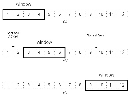
Viewing all 761 articles
Browse latest View live